
Does anyone recall struggling with math problems in high-school? We are talking specifically about the problems in coordinate geometry, where you need to solve a set of equations for a curve in order to find tangents, intersections etc. There is one class of equations, that always seemed to turn up in coordinate geometry and that is the equation of conic curves, which have this general form

This equation can be used to represent a circle, ellipse, parabola and a hyperbola.
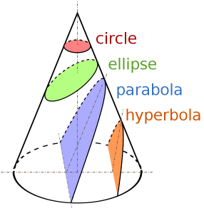
“A conic section is a curve obtained by the intersection of a plane and a circular cone. Depending on the angle of the plane with respect to the cone, a conic section may be a circle, an ellipse, a parabola, or a hyperbola.”
Now here’s a math problem for you – “Suppose you are given a set of 10 points. How would you find out the type of conic curve that these points represent?” How would you do it? You might be thinking of writing lots of equations! That sounds like a tough problem!

What if we told you that there is no need to solve this problem analytically yourself (using equations), but rather you can use a machine learning algorithm “to learn the equations for identifying a conic section”
Sounds exciting, doesn’t it? We’ll show you how it’s done.

We will show you how to quickly recognize any conic section shape (circle, ellipse, parabola and hyperbola) from a few sets of point coordinates.
First, let’s talk a bit about machine learning.
“Machine Learning is a field of study that involves techniques to get computers to learn from data progressively without being explicitly programmed. It is used for tasks that are too complex for humans to code directly. So instead, we provide a large amount of data to a machine learning algorithm and let the algorithm work it out by exploring that data and searching for a model that will achieve what the programmers have set it out to achieve.”
And this is what we intend to do. We will be following a supervised learning approach to build a machine learning classifier. A supervised learning technique – is where a computer is presented with examples of inputs and their desired outputs. The goal of the computer is to learn a general formula which maps inputs to outputs.
In this blog we will show you how to create a dataset of conic curves, as well as how to train a machine learning classifier to identify curve types.
Let’s tackle this problem step-by-step.
- Operating System (Windows 8/10/Linux)
- Python 3.6
- Pandas
- Numpy
- Matplotlib
- Jupyter notebook
- Scikit-learn
- TensorFlow
- Keras
Follow these instructions to set up:
pip install jupyter
pip install pandas
pip install numpy
pip install matplotlib
pip install scikit-learn
pip install tensorFlow
pip install keras
We will be writing our code in jupyter, which is an awesome application used by data-scientists and machine learning practitioners. You may think of it as an IDE for quickly prototyping code. To start jupyter, type the following in a terminal:
jupyter notebook
Create a python 3 notebook and then you can start writing your code in the cells provided. You may refer this nice jupyter notebook tutorial to get started with jupyter.
STEP 2: Generating the Dataset

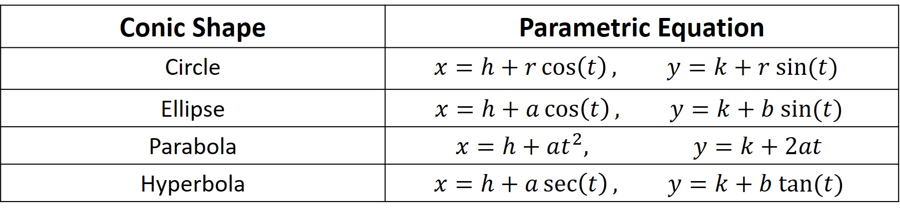
def createParabola(focal_length, centre, rotation):
    t = np.linspace(-math.pi, math.pi,100)
    x_parabola = focal_length * t**2
    y_parabola = 2 * focal_length * t
    if rotation is not None:
        x_parabola, y_parabola = rotateCoordinates(x_parabola, y_parabola, rotation)
    x_parabola = x_parabola + centre[0]
    y_parabola = y_parabola + centre[1]
    return x_parabola, y_parabola

def createCircle(radius, centre):
    theta = np.linspace(0, 2*math.pi,100)
    x_circle = radius * np.cos(theta) + centre[0]
    y_circle = radius * np.sin(theta) + centre[1]
    return x_circle, y_circle

def createEllipse(major_axis, minor_axis, centre, rotation):
    theta = np.linspace(0, 2*math.pi,100)
    x_ellipse = major_axis * np.cos(theta)
    y_ellipse = minor_axis * np.sin(theta)
    if rotation is not None:
        x_ellipse, y_ellipse = rotateCoordinates(x_ellipse,y_ellipse, rotation)
    x_ellipse = x_ellipse + centre[0]
    y_ellipse = y_ellipse + centre[1]
    return x_ellipse, y_ellipse

def createHyperbola(major_axis, conjugate_axis, centre, rotation):
    theta = np.linspace(0, 2*math.pi,100)
    x_hyperbola = major_axis * 1/np.cos(theta) + centre[0]
    y_hyperbola = conjugate_axis * np.tan(theta) + centre[1]
    if rotation is not None:
        x_hyperbola, y_hyperbola = rotateCoordinates(x_hyperbola, y_hyperbola, rotation)
    x_hyperbola = x_hyperbola + centre[0]
    y_hyperbola = y_hyperbola + centre[1]
    return x_hyperbola, y_hyperbola

def rotateCoordinates(x_data, y_data, rot_angle):
    x_ = x_data*math.cos(rot_angle) - y_data*math.sin(rot_angle)
    y_ = x_data*math.sin(rot_angle) + y_data*math.cos(rot_angle)
    return x_,y_
def plotter(x_data, y_data, title):
    fig = plt.figure(figsize=[10,10])
    plt.plot(x_data,y_data,'b--')
    plt.xlabel('X-axis',fontsize=14)
    plt.ylabel('Y-axis',fontsize=14)
    plt.ylim(-18,18)
    plt.xlim(-18,18)
    plt.axhline(y=0, color ="k")
    plt.axvline(x=0, color ="k")
    plt.grid(True)
    saveFile = title + '.svg'
    plt.savefig(saveFile)
    plt.show()
x,y = createParabola(focal_length= 1, centre= [10,10],rotation= math.pi/5)
get_n_samples(x,y, sample_count)
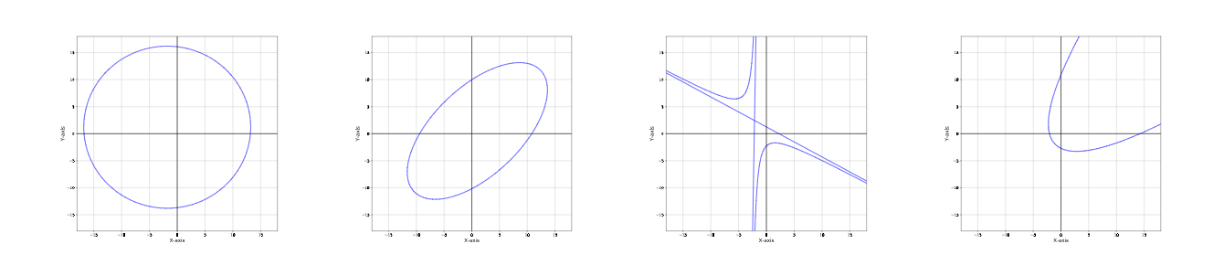

We will store variations of each parameter in separate lists. The below code snippet creates a list of 100 uniformly spaced values for each parameter, in a specified interval.
# Parabola
focal_length_array = np.linspace(1, 20, 100)
centre_x_arr = np.linspace(-12, 12, 100)
centre_y_arr = np.linspace(-12, 12, 100)
rotation_array = np.linspace(2*math.pi, 100)
To define a curve, we will choose a random parameter value from each of the above parameter lists.
Once the parameters for a curve have been chosen and the curve points have been generated, we sample 6 points uniformly from the generated curve.
sample_count = 6
parabola_dataset = pd.DataFrame()
for i in range(1000):
    focal_length = focal_length_array[get_random_index(len(focal_length_array))]
    centre_x = centre_x_arr[get_random_index(len(centre_x_arr))]
    centre_y = centre_y_arr[get_random_index(len(centre_y_arr))]
    rotation = rotation_array[get_random_index(len(rotation_array))]
    x,y = createParabola(focal_length= focal_length, centre= [centre_x, centre_y],rotation= rotation)
    x_, y_ = get_n_samples(x, y, sample_count)
    data = build_dataset(x_, y_, 'parabola')
    parabola_dataset = parabola_dataset.append(data, ignore_index=True)
We can do this similarly for the other curve types as well. You can refer to this notebook that contains all the code to see how the rest of the curves have been generated.
We now have a dataset of 4000 curves that contains 4 types of conic curves, created using different sets of parameters along with rotation and translation. Here are a few samples of the curves that have been generated :
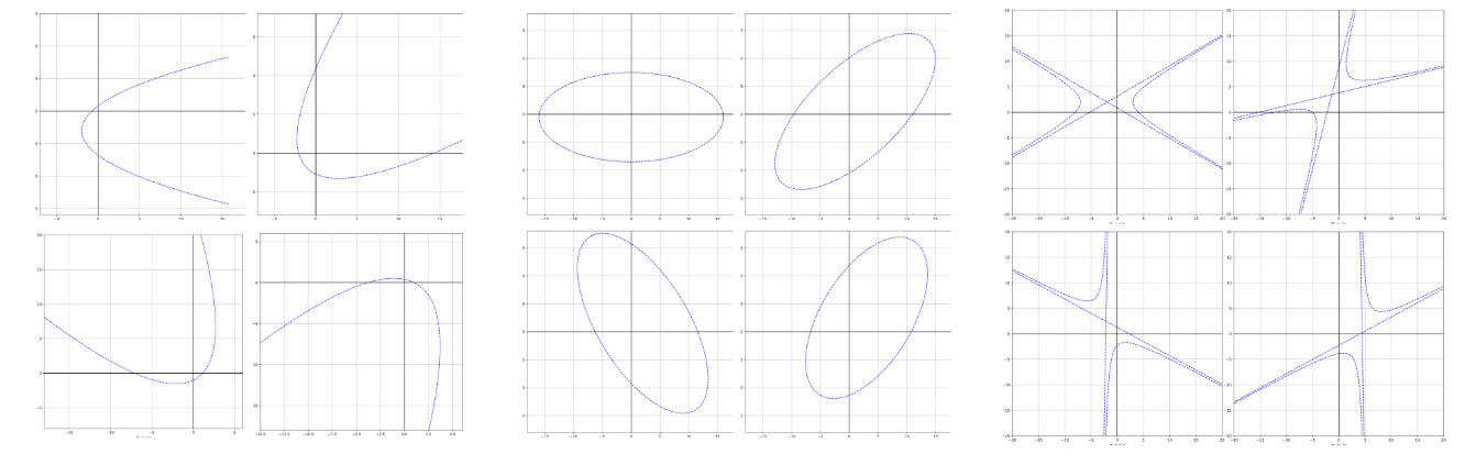
Export the data of all curves into a single csv file. We will leave this as an exercise for you.
(Hint: Pandas provides a really nice interface to do so)
STEP 3: Training a Machine Learning Algorithm
data = pd.read_csv('Conic-Section_dataset.csv', index_col=False)
data= data.sample(frac=1, random_state=42).reset_index()
data.drop(['index'], 1, inplace=True)

Let’s process out data first by converting the string labels (‘circle’ / ‘parabola’ / ‘ellipse’ / ‘hyperbola’) into integer values. Why do we need to do this? It’s because the machine learning algorithm is mathematical, and strings don’t mean anything to it!
We will convert our labels into integer values. Since we have four classes, we will get four integer values (0,1,2,3). To convert to integer values, we use the LabelEncoder class from scikit-learn.
X = data.values[:,1:]
Y = data.values[:,0]
# encode class values as integers
encoder = LabelEncoder()
encoder.fit(Y)
encoded_Y = encoder.transform(Y)
# convert integers to dummy variables (i.e. one hot encoded)
dummy_y = np_utils.to_categorical(encoded_Y)
Y : [“parabola” , “ellipse” , “circle” , “hyperbola”]
Into this
encoded_Y : [0 , 1 , 2 , 3]
Which then becomes
dummy_Y : [1, 0, 0, 0] , [0, 1, 0, 0] , [0, 0, 1, 0] , [0, 0, 0, 1]
def baseline_model():
# create model
    model = Sequential()
    model.add(Dense(128, input_dim=12, activation='relu'))
    model.add(Dropout(0.2))
    model.add(Dense(256, activation='relu'))
    model.add(Dropout(0.3))
    model.add(Dense(64, activation='relu'))
    model.add(Dropout(0.5))
    model.add(Dense(32, activation='relu'))
    model.add(Dropout(0.5))
    model.add(Dense(4, activation='softmax'))
# Compile model
    Adadelta =  optimizers.Adadelta(lr = 1)
    model.compile(loss='categorical_crossentropy', optimizer=Adadelta, metrics=['accuracy'])
    return model
Finally, we are using the categorical cross entropy for computing the loss during training and an efficient optimization algorithm Adadelta for training the data set.
After compiling the model, we call the model.fit() function to start the training on our data. In the model.fit(), we specify the features and targets. We also specify that the algorithm should use 80% data for training and 20% data as unseen data(validation_split=0.2), for performing inference.
history = model.fit(x=X,y=dummy_y,validation_split=0.2,shuffle=True, epochs=200, batch_size=12)
After the model.fit() execution is complete, we obtain loss and accuracy curves for the training and validation data.
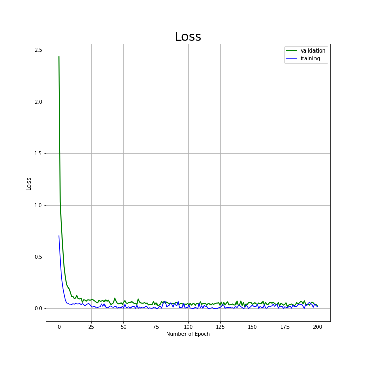
Train and Validation loss curves
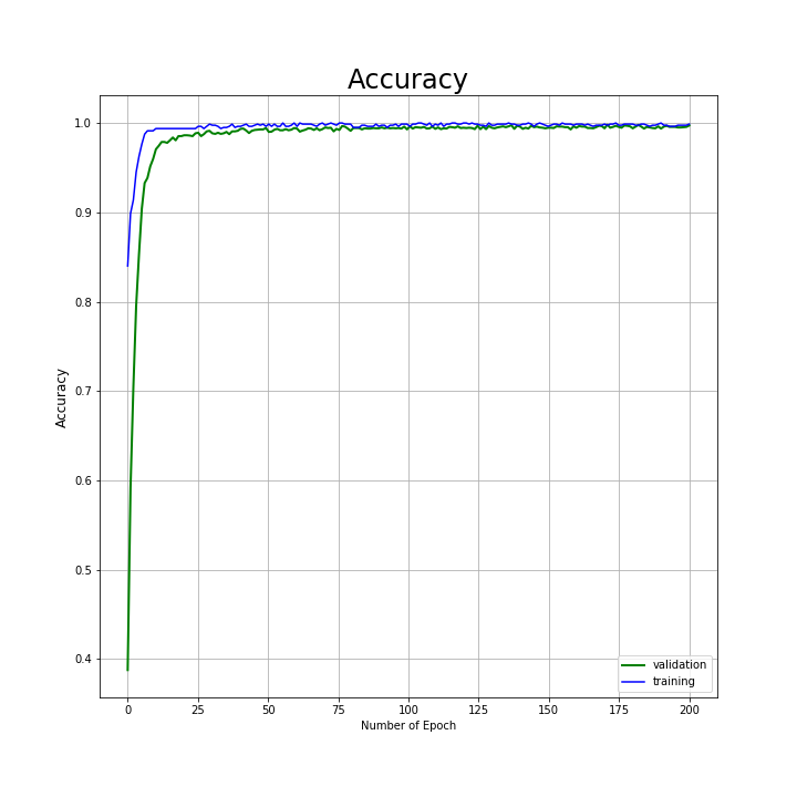
Train and Validation accuracy curves
Looking at the curves, we seem to have achieved an accuracy of 99.38% on unseen data. This means our model has learnt to distinguish conic curves like a pro!

Summary and Conclusions
We were able to build a classifier that can classify any conic curve given the six coordinates of the curve as input. And we were able to achieve a solid accuracy of 99.38% in our model.
Epoch 199/200
3200/3200 - 0s 117us/step - loss: 0.0822 - acc: 0.9922 - val_loss: 0.0311 - val_acc: 0.9935
Epoch 200/200
3200/3200 - 0s 114us/step - loss: 0.0979 - acc: 0.9878 - val_loss: 0.0167 - val_acc: 0.9938
For the benefit of our readers, we have open-sourced our notebooks for data generation as well as training on github. They can be found here : cctech-labs/ml-2dshapes
As a future experiment, we will try to do this for curves and surfaces in 3-D space. Do stay tuned to our blog, and please let us know your thoughts in the comments. Thanks for reading!